🕹 DoE or Die with Gabbar Singh
Hum ko kucch nahin pata
Gabbar Singh
Hypothesis
Design of Experiments
PPDAC Workflow
Sampling
Randomization
Introduction
Now that we know we have to ask Questions, let us ask the most famous Question of all!!
Which one? Take your pick:
- “Are O Sambha! Kitna inaam rakhe hai sarkar hum pe?”
- “To be or not to be, that is the question”
- “Hmmm…kitne aadmi thay?”
Design of Experiments
We learnt a lot (new) words from Hamlet, didn’t we? How many do we remember? What do we have a hunch about? What Hypothesis could we make? Let us pretend we are with Hamlet, and design a simple experiment to find out some “truth” (highly probable idea) that is important to us. And then we will travel to Ramgadh and get help from Gabbar Singh!
Problem / Hypothesis Design
Let us consider the Short Term Memory (STM) of Foundation Students at SMI as our vehicle for testing similar Hypotheses. This here is a paper describing a simple Design of Experiments workshop in class much like ours. We will use it to guide our Hypothesis Testing and the Design of our Experiment. We will try to mimic as much of this as we can. Do read through this in the evening today in preparation for our experiment.
In this paper, the class devises a Short Term Memory(STM) test tool, which measures the STM of a set of people randomly chosen as respondents.
Alternatively, we could use the Guilford Alternative Uses Creative Test, which is a General Creativity Test for Divergent Thinking). With the Guilford Divergent Thinking Test, you might consider:
- Students who speak their Mother Tongue fluently score better in Divergent Thinking Scores (Fluency, Flexibility, Elaboration, Originality)
- There is a significant difference in Guilford Scores between students from “small towns” and those from metros.
What Questions might we think of, to form our Hypotheses (plural!)? Questions usually are formulated in the following manner:
NoteHypothesis Sample Format
Are STM scores significantly different, on average, when [some factor] is varied between two levels?
For example:
Are STM scores significantly different:
- Art vs Design: between students of Design and those of Art? (;-O)
- Windows vs Macs: between students who use Windows as compared to those who use Macs (;-O)
- No. of Words (Few / Many): when using a short list vs a long list of words
- Word complexity: when the number of Syllables are few or large in number?
- Exposure Time ( Long / Short): when the list is shown to the resondent for a long or a short time?
- Recall Time ( Long / Short): when the time given to the respondent to recall is short or long?
Note that the last three Hypotheses are about the Test Tool Type, whereas the first two are about the population. Both types of variables are called factors. We will discuss how to deal with these shortly, both in Data Design and in Analysing the Data.
ImportantFactors are Axes
Each of the (binary) factors defines an independent axis! The combination of these axes defines a space in which we can conduct our experiment. The more factors we have, the more complex the space becomes. For example, if we have three binary factors, we have a 3D space with 8 corners (2^3 = 8 combinations). Each corner represents a unique combination of factor levels.
In each of these Hypotheses, we can see that there are binary (Yes/No) (two-valued) factors / parameters that are part of the test: Art vs Design, Windows vs Mac; and others that are inside the test tool itself: Long vs Short List of Words, Short vs Long Words and Long vs Short Exposure.
If we want our experiment to be fair we must have:
- (
Factorial ExperimentakaBlocking): Devise a Test Tool Type for each combination of binary parameters (\(2^n\) for \(n\) binary factors!!! Gasp!!) - (
Replication): The same number of respondents for each Test Tool Type - (
Randomization): Randomly select the people as respondents each Test Tool Type
We can see this can become exponentially hard if we choose say more than 3 binary factors. Let us do that!!
Data Design
What will our data look like then? We want to evaluate multiple STM scores for each setting of the binary factors. Accordingly, our Data format might look like this:
Here, in Table 1, we have (only) 8 respondents, each with a unique combination of the three binary factors. Each respondent has an associated STM score. To ensure replication, we would of course need to have more respondents for each combination of the three binary factors.
Analysis Design
We want to be able to state a clear inference/conclusion for each of the factors. We have three binary factors, and these are all independently settable. How do we compute the effect for just one of them?
ImportantFlattening the Experiment Space
Our experiment space is a cube. In order to compute the different in average scores between the two setting of any binary factor, we need to flatten / collapse the cube onto just that axis, so that we can compare the two settings of that factor.
Now that we have just two levels, we take the average on both ends and decide if that is big enough for us to think that this factor makes a difference to STM scores. ( i.e. has an effect)
And identically with the other factors.
Let us now explore two very different methods to decide whether each factor has an effect.
Data Analysis-1: Comparison of STM Histograms using Excel and WTFcsv
We do this flattening of the data cube by stacking the scores from all the other factors together, so that we have just two columns of scores, one for each setting of the factor under consideration. This allows us to compute the difference in average scores between the two settings of that factor, while controlling for the other factors.
Once our test/survey is complete, let us collate all the data for all tests using this Excel spreadsheet, which we can place on Google Drive for the whole class. (This is for the STM Hypothesis; we can adapt this spreadsheet for any other hypothesis test with categorical factors and scores.)
- Enter the data from all tests on the first sheet titled “RawData” (the one with the warning)
- Download and save as your own named local copy.
- Duplicate this data on the sheet titled “Data Duplicated”. Do not touch the “RawData” sheet again. Good Practice to never touch original data!!
- For each of the factors under consideration, we will need to stack up STM scores from \(2^3 = 8\) tests, i.e. eight columns.
- If we have three two-valued, categorical factors, we will get thres sets of stacked scores, each from a (shuffled) set of the tests.
- Half the scores in these stacked columns will pertain to one level of the factor, and the other half of the scores will pertain to the other level. (This should remind you of the Karnaugh Map you may have learnt in your digital logic courses in school.). See example below: it shows how we can stack up the scores from 4 tests for each level of the parameter p1.
| test | p1 | p2 | p3 | scores |
|---|---|---|---|---|
| A | True | Long | Big | 20 |
| B | True | Long | Small | 20 |
| C | True | Short | Big | 20 |
| D | True | Short | Small | 20 |
| E | False | Long | Big | 20 |
| F | False | Long | Small | 20 |
| G | False | Short | Big | 20 |
| H | False | Short | Small | 20 |
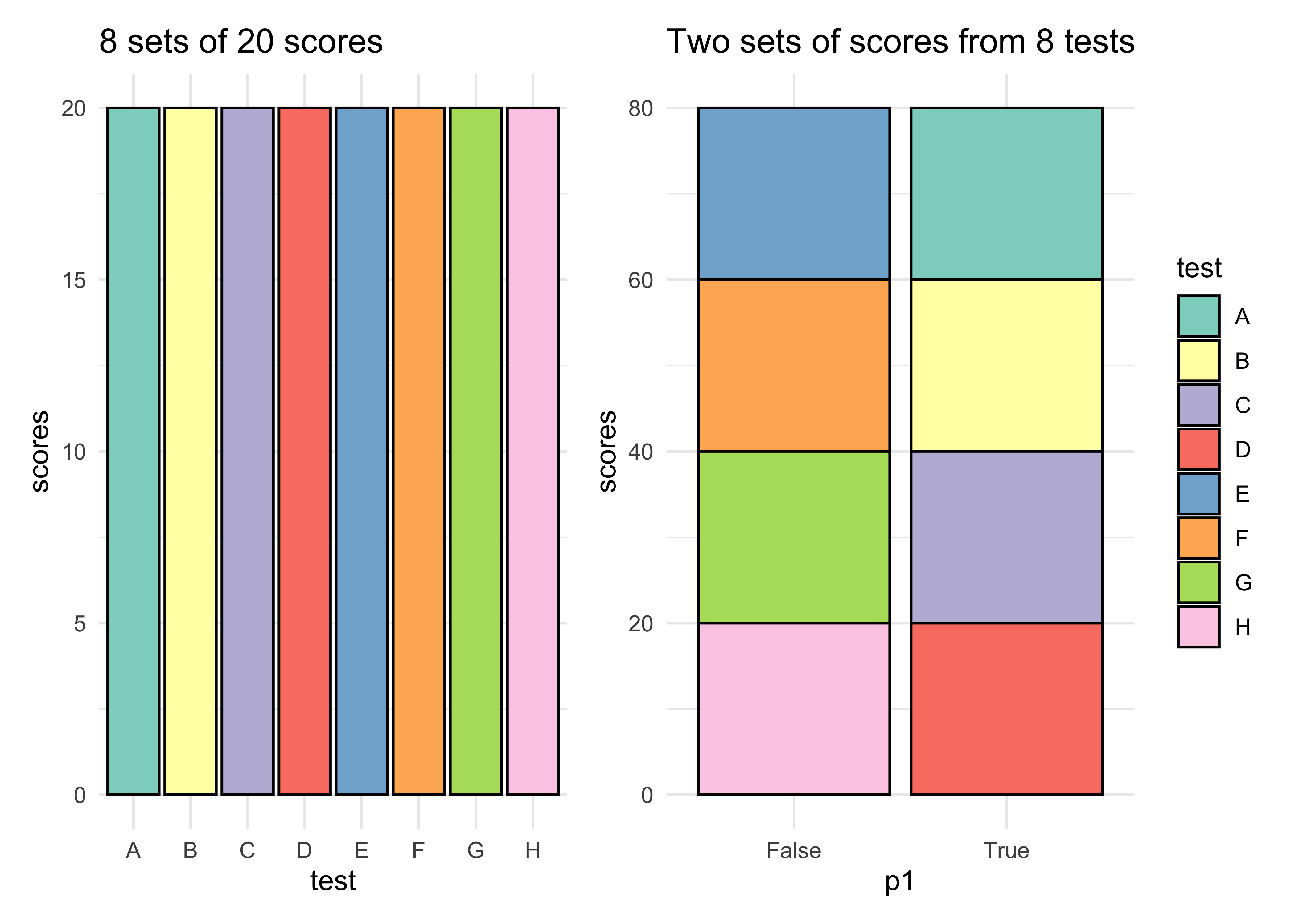
- We will set up each of these two stacked-score columns in Col A on separate sheets, similar to the one shown in the sheet titled “Permutation Test”. One sheet for each two-valued parameter.
- Create paired Histograms for each of the two stacked-score columns using WTFcsv, or Excel itself if you are confident. Ensure that there are TWO Histograms: one for each value of the factor under consideration.
- Inspection of the shapes and locations of these paired Histograms may give you an idea whether the factor under consideration has any effect on STM scores or none.
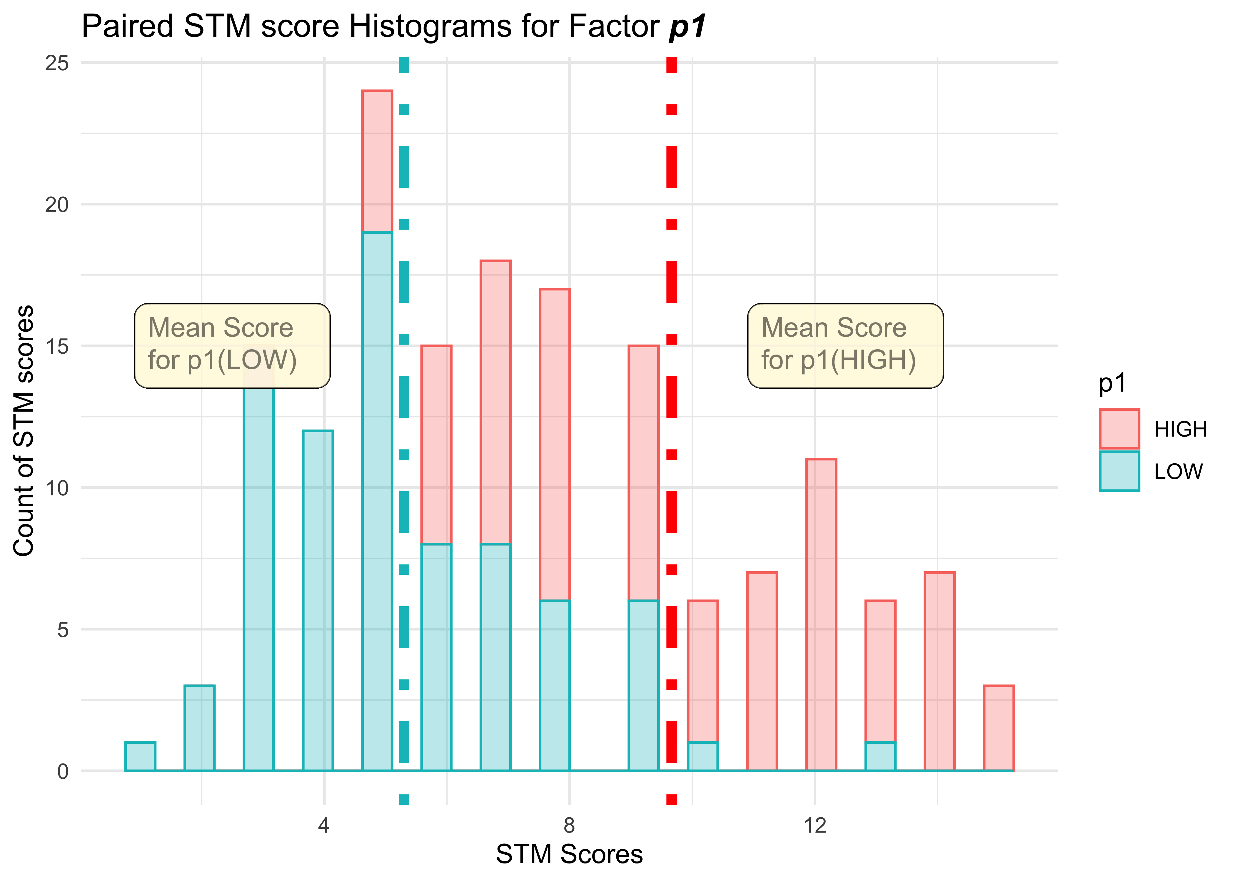
- Save these 6 histograms as PNG files on your machines and use them along with Comic Generator (discussed below) to tell the story of your Hypothesis Testing.
Data Analysis-2: Computing Parallel Worlds with Gabbar Singh
BTW, why did Gabbar Singh say to Kaalia and the others in Sholay, “Hum ko kuchh nahi pata”? And then afterwards, “Kamal ho gaya”…why does he say that?
What if we cannot trust our eyes to compare the pair-wise Histograms? If there was considerable overlap? Is there a better way? Can we fix this by playing another Childhood Game? Yes, with a deck of cards! But before we play with cards, some background: first, the immortal Gabbar Singh:
A. Gabbar Singh performs a Permutation Test.
Let us treat the three dacoits as “units,” the three blanks vs. three bullets as a fixed set of “labels,” and imagine repeating the entire three-pull sequence many times under random spins to build a distribution of “number of survivors.” Then ask how surprising “3 survivors” is. This would be a permutation-style randomization test!
In our Experiment, scores (after squashing the cube twice) are labelled as “Long List” or “Short List”; i.e. the two levels of the chosen binary factor. By swapping labels randomly, we are mechanizing our disbelief that the scores are affected by the test-configuring label.
B. What Teachers Should Know About the Bootstrap
And more formally, Tim Hesterberg:
From:
Gabbar SinghTim C. Hesterberg (2015) What Teachers Should Know About the Bootstrap: Resampling in the Undergraduate Statistics Curriculum, The American Statistician, 69:4, 371-386 DOI: 10.1080/00031305.2015.1089789
Student B. R. was annoyed by TV commercials. He suspected that there were more commercials in the “basic” TV channels, the ones that come with a cable TV subscription, than in the “extended” channels you pay extra for. To check this, he collected the data shown in Table 1. He measured an average of 9.21 minutes of commercials per half hour in the basic channels, vs only 6.87 minutes in the extended channels. This seems to support his hypothesis. But there is not much data—perhaps the difference was just random. The poor guy could only stand to watch 20 random half hours of TV. Actually, he didn’t even do that—he got his girlfriend to watch half of it. (Are you as appalled by the deluge of commercials as I am? This is per half-hour!)
[1] 2.3459| basic | extended |
|---|---|
| 6.950 | 3.383 |
| 10.013 | 7.800 |
| 10.620 | 9.416 |
| 10.150 | 4.660 |
| 8.583 | 5.360 |
| 7.620 | 7.630 |
| 8.233 | 4.950 |
| 10.350 | 8.013 |
| 11.016 | 7.800 |
| 8.516 | 9.580 |
The average difference in ad times between the two sets of TV channels is 2.34.
How easy would it be for a difference of 2.34 minutes to occur just by chance? To answer this, we suppose there really is no difference between the two groups, that “basic” and “extended” are just labels. So what would happen if we assign labels randomly? How often would a difference like 2.34 occur?
We’ll pool all twenty observations as shown in Table 3. Then we randomly allocate half of them to label “basic” and label the rest “extended”, and compute the difference in means between the two (shuffled ) groups. We’ll repeat that many times, say five thousand times, to get the permutation distribution shown in Figure 7.
| channel | times |
|---|---|
| basic | 6.950 |
| extended | 3.383 |
| basic | 10.013 |
| extended | 7.800 |
| basic | 10.620 |
| extended | 9.416 |
| basic | 10.150 |
| extended | 4.660 |
| basic | 8.583 |
| extended | 5.360 |
| basic | 7.620 |
| extended | 7.630 |
| basic | 8.233 |
| extended | 4.950 |
| basic | 10.350 |
| extended | 8.013 |
| basic | 11.016 |
| extended | 7.800 |
| basic | 8.516 |
| extended | 9.580 |

The observed statistic 2.34 is also shown; the fraction of the distribution to the right of that value (≥ 2.34) is the probability that random labeling would give a difference that large. In this case, the value of this probability ( area coloured in green ) is 0.0046009, and is < 0.005.
It would be rare for a difference this large to occur by chance. We have randomly tried “all possible chances” and are hardly able to achieve similar, and the rarer something is, the more likely that there is an underlying truth.
And therefore we conclude there is a real difference between the groups and that ad time is different between
basicandextendedTV channels.
Data Analysis-2: The Card Trick: Creating Parallel Worlds
- We will execute on Permutation Test on one sheet step by step and decide whether that factor had a significant effect on STM scores.
- We pretend that there is no difference in scores whether the factor is chosen on way or another.
- We mechanize this pretence by lumping “both kinds” of scores together and shuffle them and divide them, randomly into two groups, and take the difference in scores.
- We can do this, like we did with our Monte Carlo experiment, many many times and calculate difference in scores each time. (It is like inventing many parallel worlds)
- If we look at the way these randomly computed scores are distributed and compare with the one measurement we did see, we can decide whether Mother Nature is up to something, or we are able to mimic the Mom.
- If we are not able to mimic Mom, then Mom always knows and we bow to her and ascribe a significance to the factor under consideration. Else, nope.
- Replicate this test for the other (binary) factors.
OK, who would like to Propose a Procedure for this, using nothing but a deck of cards?
Apropos: And how could we do this for non-binary factors …??!!!
Making a Data Comic out of our Experiment
What have been our Conclusions with the Experiment? Let us take our Experiment and make a comic out of it: Data Comic Generator from Gramener (Weblink).
References
-
Randomized Trials:
Randomized Trials David Spiegelhalter (2019) The Art of Statistics: Learning from Data, Basic Books, New York, NY, USA.
Derek Rowntree (2018) Statistics Without Tears: A Primer for Non-Mathematicians, Penguin Books, London, UK.
David Deutsch (2011) The Beginning of Infinity: Explanations that Transform the World, Penguin Books, London, UK.
Victoria Woodard (2023) Five Hands-on Experiments for a Design of Experiments Course, Journal of Statistics and Data Science Education, 31:3, 225-235, DOI: 1.1080/26939169.2023.2195889. PDF
Tim C. Hesterberg (2015). What Teachers Should Know About the Bootstrap: Resampling in the Undergraduate Statistics Curriculum, The American Statistician, 69:4, 371-386, DOI:10.1080/00031305.2015.1089789. PDF
Shuttleworth, M. (2009). What is the scientific method? Retrieved from https://explorable.com/what-is-the-scientific-method
Victoria Woodard (2023) Five Hands-on Experiments for a Design of Experiments Course, Journal of Statistics and Data Science Education, 31:3, 225-235, DOI: 10.1080/26939169.2023.2195889. PDF
Tim C. Hesterberg (2015). What Teachers Should Know About the Bootstrap: Resampling in the Undergraduate Statistics Curriculum, The American Statistician, 69:4, 371-386, DOI:10.1080/00031305.2015.1089789. PDF
Shuttleworth, M. (2009). What is the scientific method? Retrieved from https://explorable.com/what-is-the-scientific-method
Mahashweta Devi, The Why Why Girl, https://www.tulikabooks.com/picture-books/the-why-why-girl-english.html,read by Sarah Dryden Peterson. https://www.youtube.com/watch?v=xNcV5DZhg4c
-
Could this song indicate what our situation might be?
Fun Stuff: Stat Lessons from Sholay
Gabbar: “Kitne Aadmi thay?
Stats Teacher: How many observations do you have? n < 30 is a joke.
Gabbar: Kya Samajh kar aaye thay? Gabbar khus hoga? Sabaasi dega kya?
Stats Teacher: What are the levels in your Factors? Are they binary? Don’t do ANOVA just yet!
Gabbar: (Fires off three rounds ) Haan, ab theek hai!
Stats Teacher: Yes, now the dataset is balanced wrt the factor (Treatment and Control).
Gabbar: Is pistol mein teen zindagi aur teen maut bandh hai. Dekhte hain kisko kya milega.
Stats Teacher: This is our Research Question, for which we will Design an Experiment.
Gabbar: (Twirls the chambers of his revolver) “Hume kuchh nahi pataa!”
Stats Teacher: Let us perform a non-parametric Permutation Test for this Factor!
Gabbar: “Kamaal ho gaya!”
Stats Teacher: Fantastic! Our p-value is so small that we can reject the NULL Hypothesis!!
Go and like this post at: https://www.linkedin.com/pulse/stat-lessons-from-sholay-arvind-venkatadri-wgtrf/?trackingId=c0b4UCTLRea6U%2Bj%2Bm4TCtw%3D%3D
More Fun Stuff: Words Belong Hamlet
Hamlet’s To be or not to be in Pidgin English Tok Pisin!
Which way this time? Me killem de finish body b’long me. Or me no do ’im? Me no savvy.
Might ’e better ’long you-me catchem this fella, string for throw ’im this fella arrow.
Altogether b’long number one bad fella, name b’long him fortune? Me no savvy.
Might ’e better ’long you-me For fightem ’long altogether where him ’e makem you-me sorry too much.
Bimeby him fall down die finish? Me no savvy.